Data Transformation Using SPSS

Introduction

In order to gain valid results from the use of parametric tests, such as an independent-samples t-test or one-way ANOVA, a common assumption is that the dependent variable is approximately normally distributed for every category of the independent variable. Unfortunately, it is not uncommon for some or all of your groups to have data that is not normally distributed. In order to continue using these parametric tests, you need to be able to apply a transformation to the data so that the previously non-normally distributed data is now normally distributed. This guide will work through the common types of non-normality and show the type of transformations that can be applied to correct for these non-normal distributions. At this stage, however, you must understand that transformations will not always be successful.

How to apply a transformation

If a dependent variable is not normally distributed for any particular category of the independent variable(s), the dependent variable needs to be transformed for all groups. That is, you cannot just transform the data for one particular group without transforming the data of all the other groups (i.e., you have to transform every value of the dependent variable). Consider the example of engagement score (the dependent variable) between genders (the independent variable) where engagement score is normally distributed for males, but not for females, as shown below:

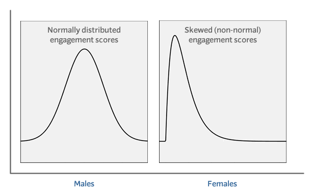
Specifically, in this case, it can be seen that engagement scores for females are positively skewed. Now, although it is only the distribution of the female engagement scores that is a problem, the entire engagement variable will have to be transformed. Transforming data in this manner can have negative consequences because while the transformation might successfully work on the category with non-normal data, when applied to data that is already normal (e.g., for males), it can turn a normal distribution into a non-normal distribution! Unfortunately, this is one of the consequences of transforming data. You either have to choose a different transformation or accept that your data cannot be completely normally distributed.

Performing transformations in SPSS Statistics

In order to perform any transformation in SPSS Statistics, you first need to open the Compute Variable dialogue box:

Click Transform > Compute Variable… on the main menu, as shown below:

You will be presented with the Compute Variable dialogue box, as shown below:

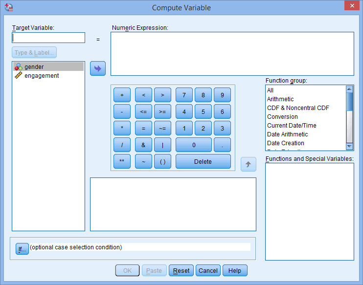
The Compute Variable dialogue box works as follows:

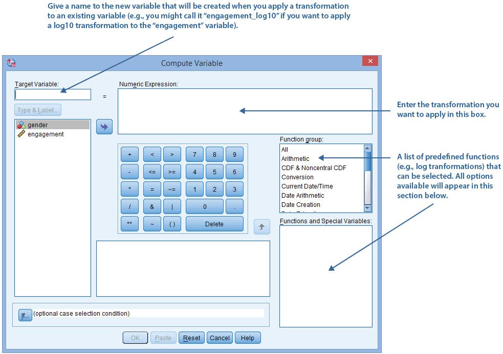
Depending on what you enter into the Numeric Expression: box will determine the transformation that is performed. It is best never to overwrite your original data, so you should create a new variable to store the new values for the transformed variable. You will have used one or more methods of assessing normality to understand that your data is not normally distributed. In order to assess the success of your transformations, you need to use the same methods of assessment you used initially, this time to re-test for normality. Different transformations have different success rates for different types of violations of normality. The following sections describe the type of normality violation and the transformation you should consider first to correct for the non-normal data. The example used below will involve transforming a variable called engagement.

Moderately, positively skewed data

To convert moderately positively skewed data to normality, you should first attempt to apply a “square root” transformation. Basically, take the square root of the scores of the variable to be transformed. Type the following into the Compute Variable box (creating a new variable called engagement_sqrt):

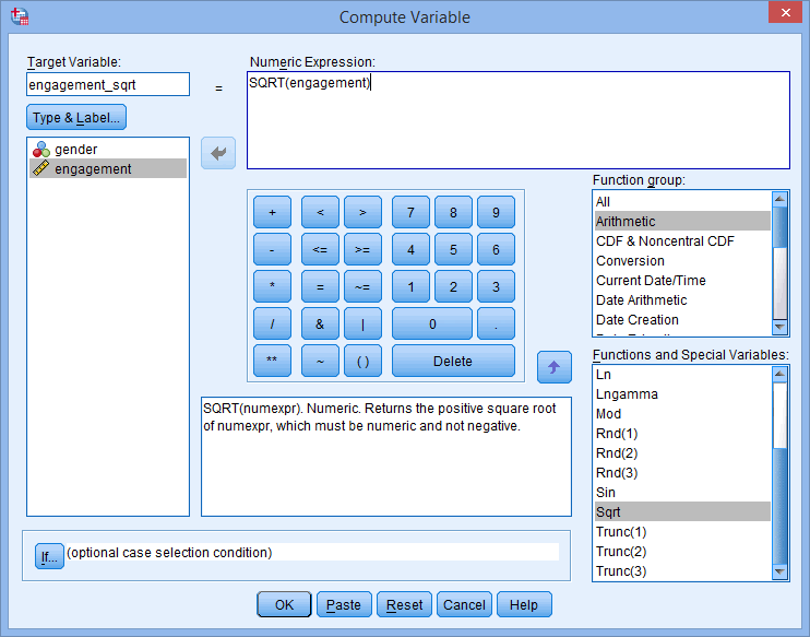
You can directly type in “SQRT(engagement)” into the Numeric Expression: box. Alternatively, you can first select “Arithmetic” from the Function group: menu, followed by selecting “Sqrt” from the Functions and special variables menu. Then double-click “Sqrt”, which will transfer this function into the Numeric Expression: box. Next, double-click on engagement, which will transfer this variable into the “SQRT()” function.

In either case, to compute the new variable, click the button.

Moderately, negatively skewed data

To convert moderately negatively skewed data to normality, you should first attempt to apply a “reflect and square root” transformation. Basically, you first need to find the largest engagement score in your data set – in this example, it is 7.23 – and then add 1 to its value. In this example, this would be 8.23. Each score then needs to be subtracted from this value and then the square root of the scores taken. Type the following into the Compute Variable box (creating a new variable called engagement_sqrt_ref):

You can directly type in “SQRT(8.23 – engagement)” into the Numeric Expression: box. Alternatively, you can first select “Arithmetic” from the Function group: menu, followed by selecting “Sqrt” from the Functions and special variables menu. Then double-click “Sqrt”, which will transfer this function into the Numeric Expression: box. Type in 8.23 and then double-click on “engagement”, which will transfer this variable into the “SQRT()” function.

In either case, to compute the new variable, click the button.

Strongly, positively skewed data

To convert strongly positively skewed data to normality, you should first attempt to apply a “logarithmic” transformation. Basically, take the log10 of the scores of the variable to be transformed. Type the following into the Compute Variable box (creating a new variable called engagement_log10):

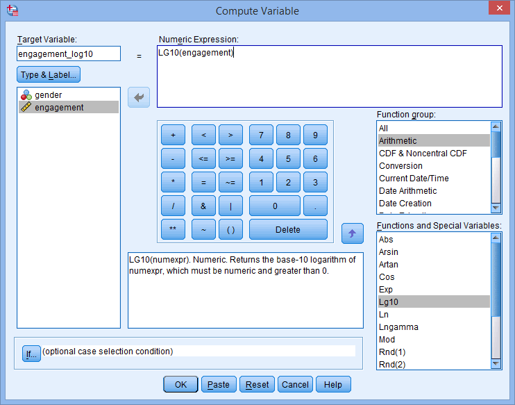
You can directly type in “LG10(engagement)” into the Numeric Expression: box. Alternatively, you can first select “Arithmetic” from the Function group: menu, followed by selecting “Lg10” from the Functions and special variables menu. Then double-click “Lg10”, which will transfer this function into the Numeric Expression: box. Then double-click on engagement, which will transfer this variable into the “LG10()” function.

In either case, to compute the new variable, click the button.

Strongly, negatively skewed data

To convert strongly negatively skewed data to normality, you should first attempt to apply a “reflect and logarithmic” transformation. Basically, you first need to find the largest engagement score in your data set – in this example, it is 7.23 – and then add 1 to its value. In this example, this would be 8.23. Each score then needs to be subtracted from this value and then logged. Type the following into the Compute Variable box (creating a new variable called engagement_log10_ref):

You can directly type in “LG10(8.23 – engagement)” into the Numeric Expression: box. Alternatively, you can first select “Arithmetic” from the Function group: menu, followed by selecting “Lg10” from the Functions and special variables menu. Then double-click “Lg10”, which will transfer this function into the Numeric Expression: box. Type in 8.23 and then double-click on “engagement”, which will transfer this variable into the “LG10()” function.

In either case, to compute the new variable, click the button.

Extremely, positively skewed data

To convert extremely positively skewed data to normality, you should first attempt to apply an “inverse” (or “reciprocal”) transformation. Basically, 1 is divided by the variable to be transformed. Type the following into the Compute Variable box (creating a new variable called engagement_inverse):

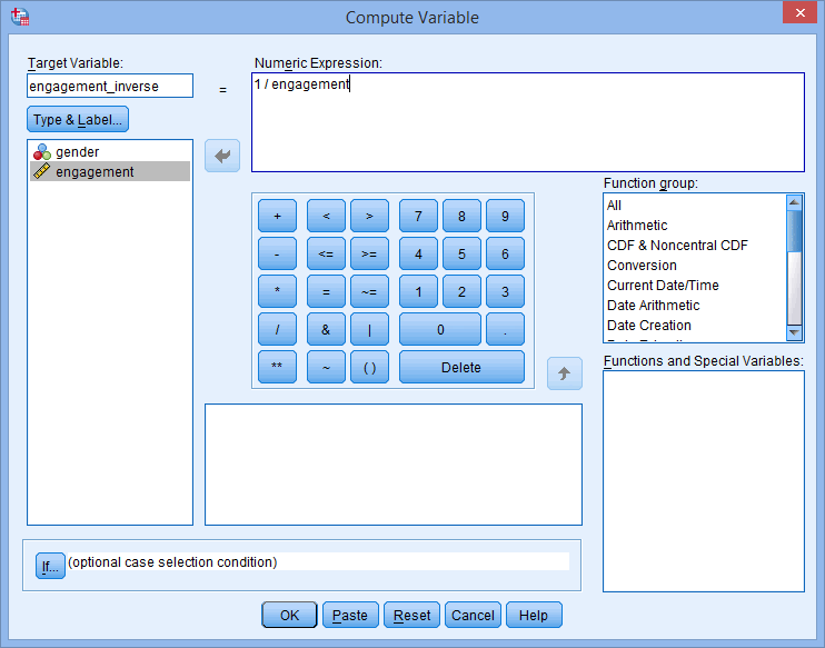
You can directly type in “1 / engagement” into the Numeric Expression: box. Alternatively, use the keypad and the list of variables on the left to transfer “engagement” to the Numeric Expression: box.

In either case, to compute the new variable, click the button.

Extremely, negatively skewed data

To convert extremely negatively skewed data to normality, you should first attempt to apply a “reflect and inverse” transformation. Basically, you first need to find the largest engagement score in your data set – in this example, it is 7.23 – and then add 1 to its value. In this example, this would be 8.23. You then subtract each score from this value. Finally, it is then 1 divided by this new value. Type the following into the Compute Variable box (creating a new variable called engagement_inverse_ref):

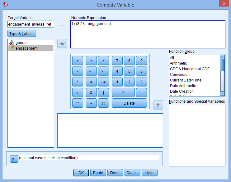
You can directly type in “1 / (8.23 – engagement)” into the Numeric Expression: box. Alternatively, use the keypad and the list of variables on the left to transfer engagement to the Numeric Expression: box.

In either case, to compute the new variable, click the button.

Linearity and heteroscedasticity

When dealing with assumptions of linear regression, it is not uncommon to need to transform data to achieve a linear relationship between variables or to make sure there is homoscedasticity. If you have a non-linear relationship, you can consider transformations of either the independent or dependent variable or both. If you have a relationship where the dependent variable starts to increase more rapidly with increasing independent variable values, you can first consider a log transformation (go to the Strongly, positively skewed data section). If your data does the opposite – dependent variable values decrease more rapidly with increasing independent variable values – you can first consider a “square” transformation. A square transformation is simply squaring the dependent variable. To do this, type the following into the Compute Variable box (creating a new variable called engagement_squared):

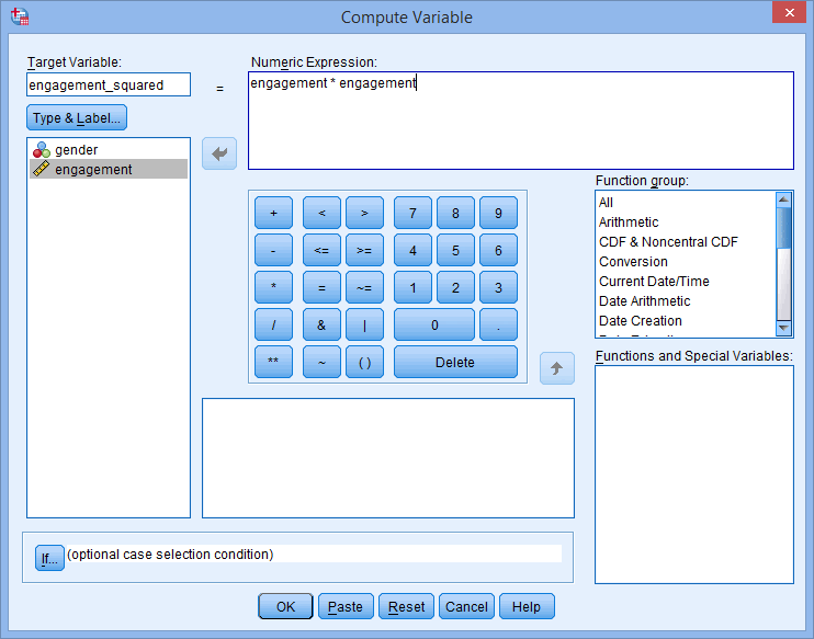
You can directly type in “engagement * engagement” into the Numeric Expression: box. Alternatively, use the keypad and the list of variables on the left to transfer engagement to the Numeric Expression: box.

If you have heteroscedasticity where the variance increases with an increasing independent variable value, you can try using a square root (see the Moderately, positively skewed data section) or logarithmic (see the Strongly, positively skewed data section) transformation on the dependent variable.